
So how much could your portfolio actually lose? That's the question Value at Risk, or VaR, tries to answer, not forever, just over a set period, at a confidence level you pick, assuming markets behave normally. Say a 1-day 95% VaR works out to ₹1,00,000. Roughly speaking, you've got a 95% shot at losing less than that in a day, and a 5% shot you don't.
One number, and it covers the whole portfolio. That's the appeal. Risk teams use it, capital planners use it, regulators ask for it. It has real flaws, we'll get to those, but you still need to know how to calculate it if you're working anywhere near market risk.
What is Value at Risk (VaR)?
Think of VaR as a statistical guess at potential portfolio loss, over a set period, at whatever confidence level you've chosen. It comes out in rupees, not as a percentage. Really it's just answering one question, dressed up in statistics: how much could I reasonably lose here, given how sure I want to be about it?
You need three pieces before the number means anything at all. An amount. A time horizon, could be a day, ten days, a month, whatever fits. And a confidence level, almost always 95% or 99%. Miss one of those and the figure's basically useless on its own. Someone tells you "VaR of ₹50,000" and, honestly, that tells you nothing. "1-day VaR of ₹50,000 at 95% confidence" though, now that actually says something.
See Also: How Can Market Mechanics Be Represented and Tested Using Quantitative Tools?
Why is VaR Important?
A portfolio can be leaking risk from a dozen directions at once, different assets, different currencies, market factors nobody's watching closely. VaR squashes all of that down into one figure, and a trader, a risk manager, and a regulator can all look at that same number and understand it the same way.
This isn't just a reporting exercise either, it drives real decisions. Capital allocation often runs on VaR: how much capital does this desk actually need against what it's risking? Risk managers lean on it to set position limits and to catch risk creeping upward before it becomes a problem. And under Basel-style banking rules, regulators have tied capital reserves to VaR numbers on the trading book for a long time now.
There's also just the plain communication side of it. Tell a board member there's a 5% chance the desk loses more than ₹2 crore this month, and they get it immediately. Put a covariance matrix in front of them instead, and watch the room glaze over.
Inputs Required to Calculate VaR
You need four things before you can calculate VaR, whichever method you use.
- Portfolio value, what the position or portfolio is worth right now.
- Volatility, usually the standard deviation of past returns, a measure of how much the value has swung around.
- Confidence level, 95% or 99% most often, how sure you want to be that losses stay under the VaR figure.
- Time horizon, the window you're measuring, a day, ten days, a month.
Got more than one asset? Add correlation to the list. Assets that don't move in lockstep bring the total risk down through diversification.
VaR Formula Explained
The parametric, or variance-covariance, method uses this formula:
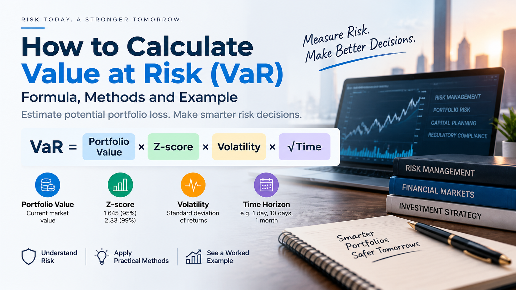
VaR = Portfolio Value × Z-score × Volatility × √Time
Here's what each piece means:
| Variable | What it means |
|---|---|
| Portfolio Value | The current market value of the position being measured |
| Z-score | A statistical value corresponding to your chosen confidence level (1.645 for 95%, 2.33 for 99%), assuming a normal distribution of returns |
| Volatility | The standard deviation of the portfolio's returns over your chosen base period, usually daily |
| √Time | A scaling factor that adjusts volatility from your base period to your desired time horizon (for example, scaling daily volatility to a 10-day horizon) |
One thing worth flagging now, before you go any further: this formula assumes returns follow a normal distribution, and they don't, not exactly. Real markets throw up what people call "fat tails", big moves showing up more often than a clean bell curve would predict. We'll come back to why that matters.
How to Calculate VaR Step-by-Step
- Determine your portfolio value: Use the current market value of the position or portfolio you're analyzing.
- Calculate historical volatility: Pull a run of historical daily returns and work out their standard deviation. That's your volatility input.
- Select your confidence level: 95% or 99%, depending on how conservative you need to be. Then grab the matching Z-score, 1.645 or 2.33.
- Choose your time horizon: One day? Ten days? Something else? Scale your volatility with the square root of time if it isn't already in the right units.
- Apply the formula: Multiply portfolio value by the Z-score, by volatility, by the square root of time.
- Interpret the result in context: State it fully, amount, time horizon, confidence level, or the number won't mean anything to whoever reads it next.
One more step if you're working with more than one asset. Before step 5, combine each asset's volatility using the correlations between them, so you get a real portfolio-level volatility instead of just adding numbers together. Assets that don't move together bring your risk down.
VaR Calculation Example
Say you're holding a ₹10,00,000 portfolio, and its daily returns have a standard deviation of 1.5%. You want the 1-day VaR at 95% confidence.
Step 1: Portfolio Value = ₹10,00,000
Step 2: Volatility = 1.5%, or 0.015
Step 3: Confidence level = 95%, so Z-score = 1.645
Step 4: Time horizon = 1 day, so √Time = √1 = 1
Applying the formula:
VaR = ₹10,00,000 × 1.645 × 0.015 × 1 VaR = ₹24,675
What that actually means: on a normal day, this portfolio shouldn't drop more than ₹24,675, and that holds 95% of the time. The other 5% of the time, it might. And if it does, don't ask this number how much worse things got, it won't tell you.
Want the 10-day figure instead? Swap in √10, which is about 3.16. That pushes VaR up to roughly ₹77,973. Makes sense, more time means more room for things to move.
Methods of Calculating VaR
Three approaches dominate here, and each one trades off differently.
| Method | How it works | Important Assumption | Best used when |
|---|---|---|---|
| Historical Simulation | Applies actual historical price changes to the current portfolio to generate a distribution of possible outcomes | Future returns will resemble the historical period used | You want a model-free approach that doesn't assume a specific statistical distribution |
| Variance-Covariance (Parametric) | Uses the formula above, based on volatility, correlation, and an assumed normal distribution | Returns are normally distributed | You need a fast, simple calculation and your portfolio's returns are reasonably close to normal |
| Monte Carlo Simulation | Generates thousands of random possible future price paths based on statistical assumptions about the portfolio's behavior | The underlying statistical model used to generate scenarios is reasonably accurate | You're modeling complex portfolios with options or non-linear instruments where simpler methods fall short |
None of them wins outright. Historical simulation sticks close to what actually happened, but it assumes the future rhymes with the past. Variance-covariance is quick and easy, until your returns stop looking normal, which happens more than people expect. Monte Carlo can handle messy, complex portfolios, but it eats computing power and lives or dies by how good your underlying model is. A lot of risk desks just run two or three methods side by side and compare notes.
Limitations of VaR
VaR is everywhere in risk management, sure. Doesn't mean it's not flawed.
- It doesn't describe tail risk: All VaR gives you is where the line sits at your chosen confidence level, nothing about what's waiting on the other side of that line. Two portfolios can post the exact same VaR number and still have completely different worst-case scenarios lurking underneath.
- It can understate risk during extreme events: Blame the normal distribution assumption baked into the parametric method, normal distributions just don't expect big, ugly moves as often as they actually happen. Real returns run fatter in the tails than the model wants to admit.
- Historical simulation assumes the past resembles the future: Except conditions shift, they always do eventually, and a model trained on old data can end up badly misreading what's happening right now. Which is basically the whole reason backtesting exists in the first place.
- It's not additive across correlated risks: Add up VaR numbers from different desks and call that your portfolio total? Don't. Correlation changes how those risks actually combine, and skip that step and you'll end up with a number that's just wrong.
Partly because of all this, Expected Shortfall, sometimes called Conditional VaR, has picked up ground alongside plain VaR. It estimates the average loss once you're past that VaR threshold, so you get a better feel for how ugly "ugly" can really get. Basel's newer market risk rules lean on Expected Shortfall now too, sometimes as a companion to VaR, sometimes as a straight replacement.
Related Concepts
VaR doesn't exist in a vacuum. Market risk and portfolio risk are really the broader things it's trying to measure. Confidence level and time horizon are the two dials you turn to define any specific VaR number. Stress testing comes at the problem from another angle entirely, running specific extreme scenarios rather than leaning on a probability distribution. Capital allocation decisions lean on VaR outputs constantly, and Basel rules have tied bank capital requirements to it for years now.